Mean-Field GameFictitious PlayNYC TLC DataBackward InductionPrice of Anarchy
Overview
What is NashCab?
We model a ride-sharing platform (Uber/Lyft) as a Mean-Field Game (MFG).
Each driver is a strategic agent who, at every minute, decides whether to
accept or reject
a randomly offered ride. Drivers don't reposition proactively — their zone changes only when they complete a trip.
We find the Mean-Field Nash Equilibrium: a joint policy from
which no driver can unilaterally deviate to earn more, given all other drivers follow the same strategy.
Assume µidle
driver distribution
→
Backward Induction
compute V, π
→
Forward Simulation
simulate all drivers
→
New µidle
emergent distribution
→
Converged?
‖µ_new − µ_old‖₁ < ε
🎯
Backward Induction
Compute V(z,t) — expected future earnings — backwards from T→0. At each step, the driver compares Q_accept vs Q_reject using a sigmoid policy.
🔄
Forward Simulation
Run all drivers forward using the computed policy π. Drivers scatter to destination zones after accepting rides, producing a new µ_idle distribution.
⚖️
Nash Equilibrium
When µ_new ≈ µ_old, we have found a fixed point. Every driver is already best-responding — no one can do better by deviating.
📉
Price of Anarchy
PoA = W_opt / W_MFNE measures welfare loss from selfish behavior. A PoA of 1.52 means drivers deliver only 66% of the socially optimal matching.
Phase 1
Synthetic Grid City
A 7×7 grid of 49 zones with synthetic demand. Three demand profiles test how
spatial structure affects equilibrium behavior and the Price of Anarchy.
49
Zones (7×7 grid)
500
Total drivers
500
Time steps T
59–139
Iterations to converge
1.37
PoA (hotspot)
31.9%
Busy fraction (hotspot)
Initialization — Warm Start
µ[z,0] = 1/500
uniform across all 49 zones
→
Always-accept sim
run T=500 steps
→
Consistent µ[z,t]
realistic trajectory for t=1…500
We start with every driver spread uniformly — 1/500 of drivers at each of the 49 zones at t=0. We can't just hold this uniform distribution for all T steps because by t=250, drivers have been moving for 250 steps and the real distribution looks nothing like uniform. Using uniform throughout would make the first backward pass compute p_offer values ~3–4× off at mid-horizon, and the outer loop never recovers. So we first run one forward simulation under an always-accept policy to get a physically consistent starting trajectory, then begin the fictitious play loop from there.
Convergence
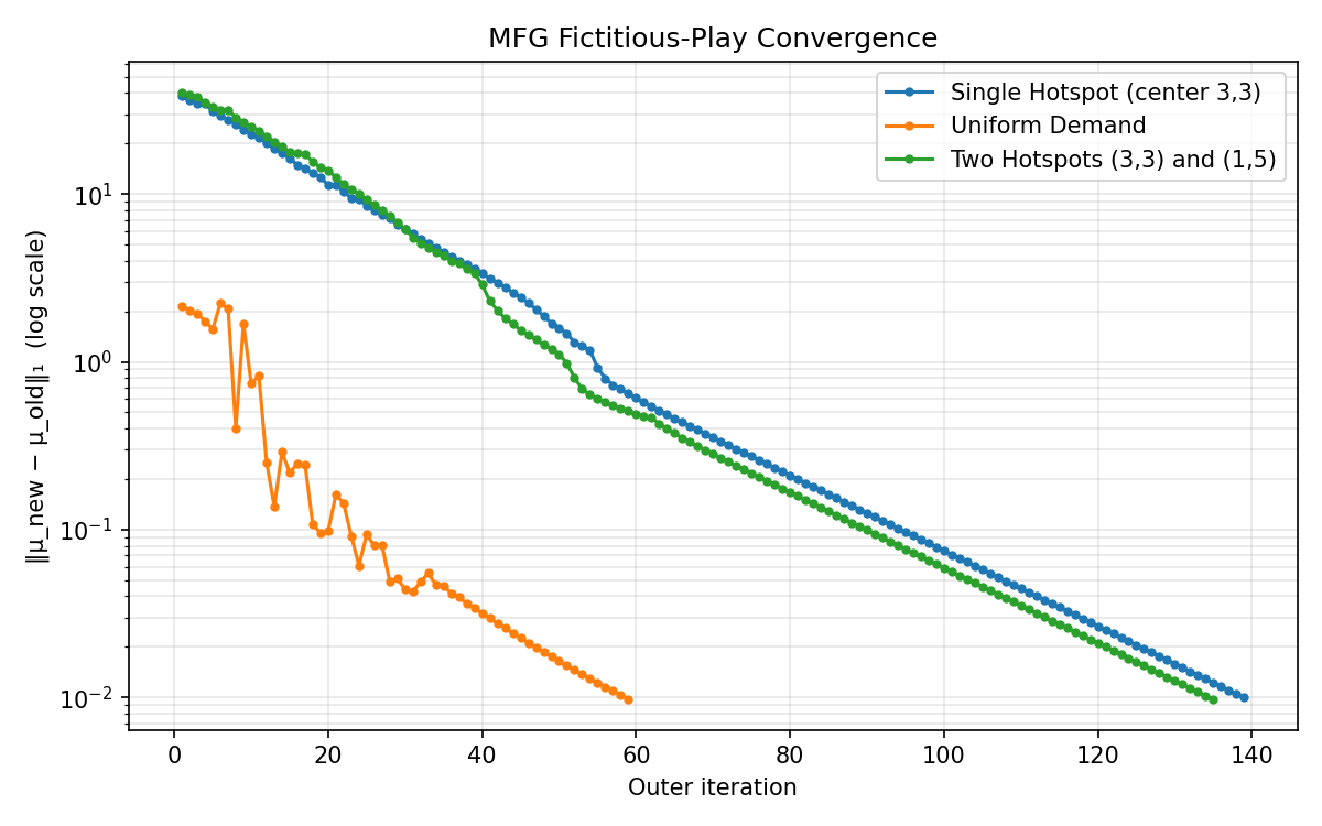
All three profiles converge with α = 0.05 and ε = 0.01. Log-linear L1 decay consistent with geometric convergence.
L1 convergence of the outer fictitious-play loop — all three demand profiles
Demand Profiles
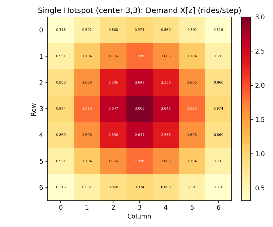
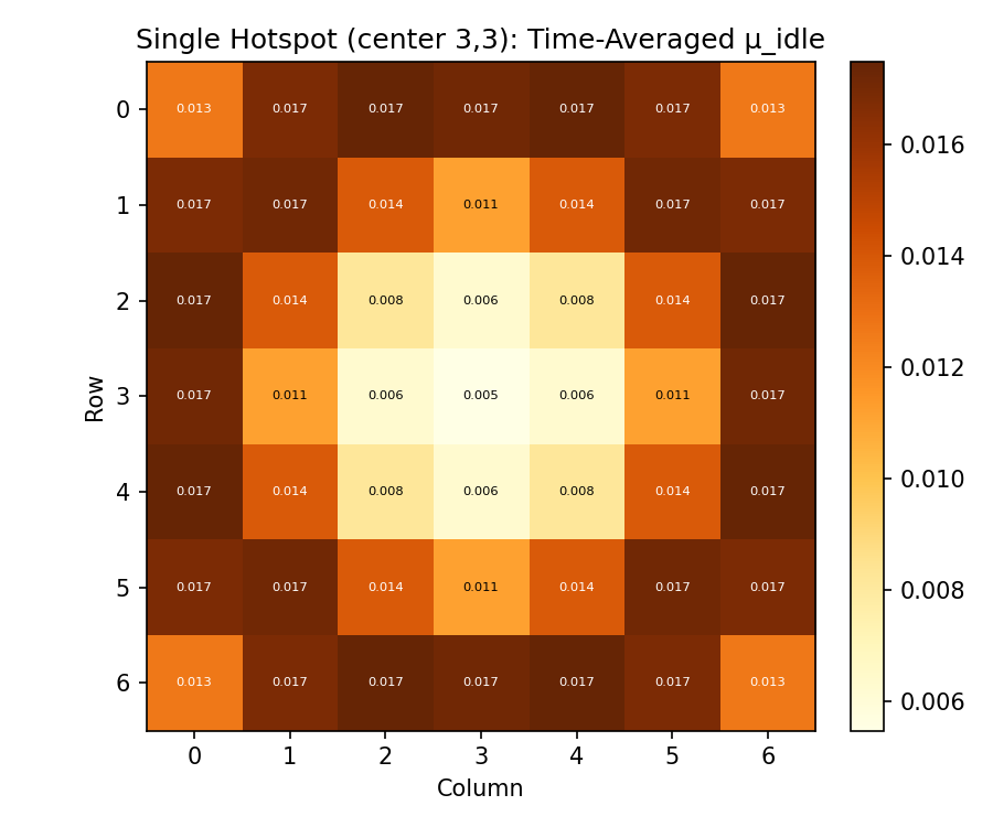
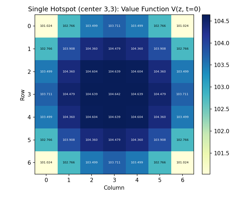
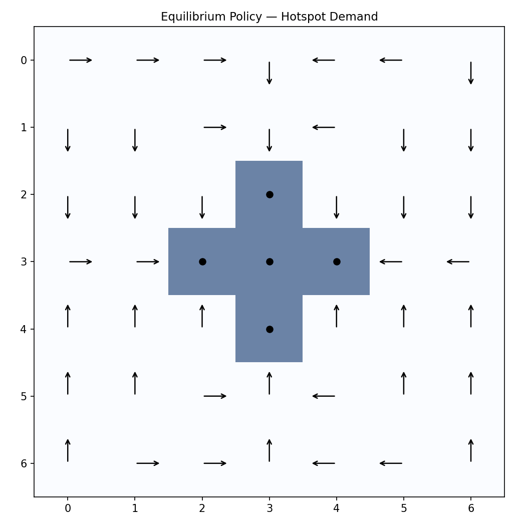
Single Gaussian demand peak at the center (3,3). Center zone is demand-saturated; edge zones rarely get offers. PoA ≈ 1.37.
Demand X[z] — Single Hotspot
Equilibrium idle distribution — center (3,3) has almost no idle drivers (demand = offers instantly), edges have the most (drivers dropped here after rides, rarely get new offers)
Value function V(z, t=0) — center zones earn more due to high offer rates
Net drift direction of accepted rides at t=0 — drivers everywhere prefer destinations toward the hotspot at (3,3), since being near high demand means more future earnings
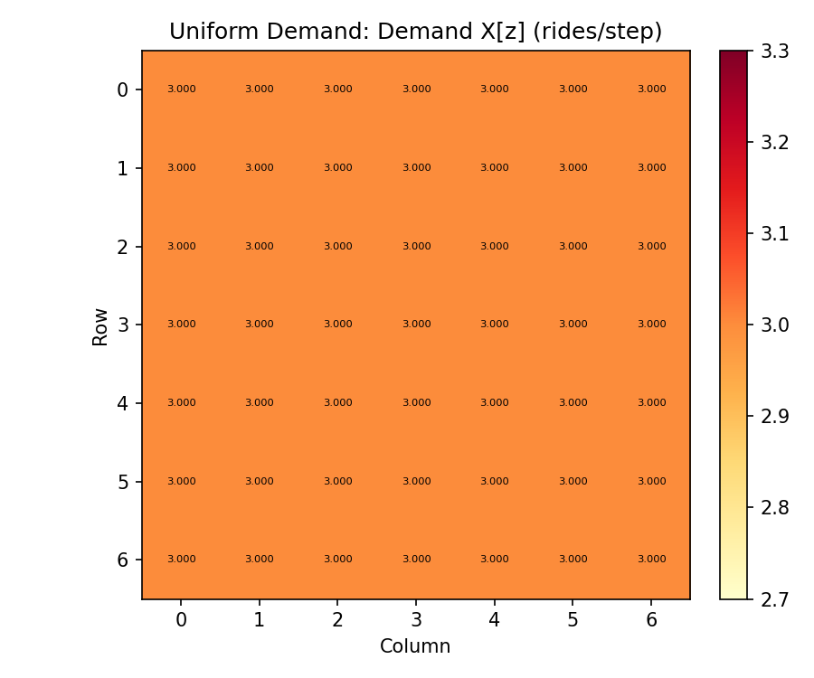
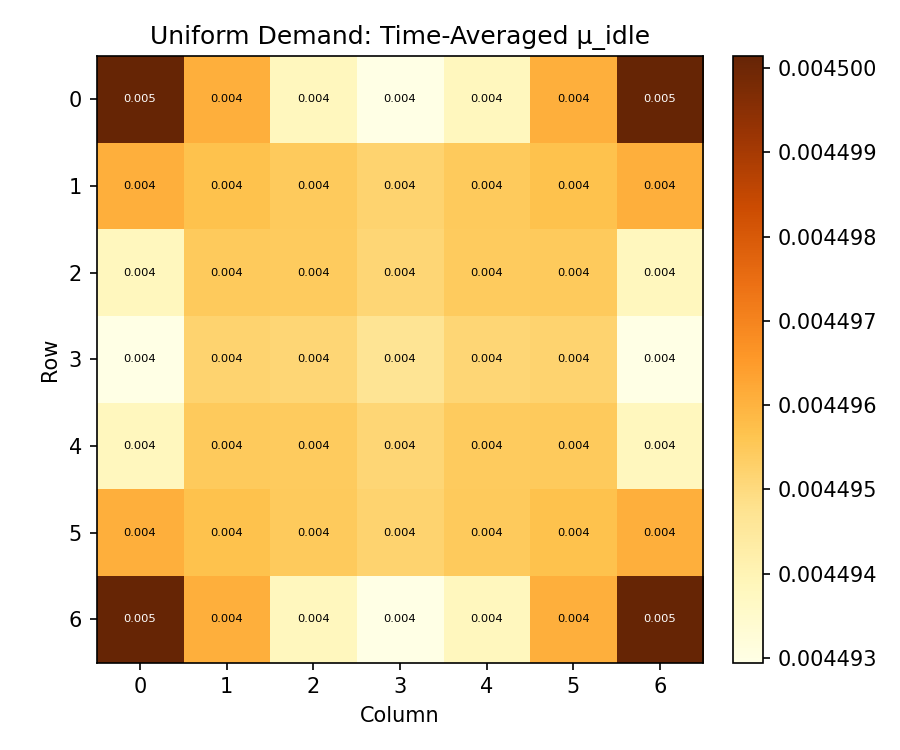
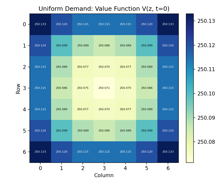
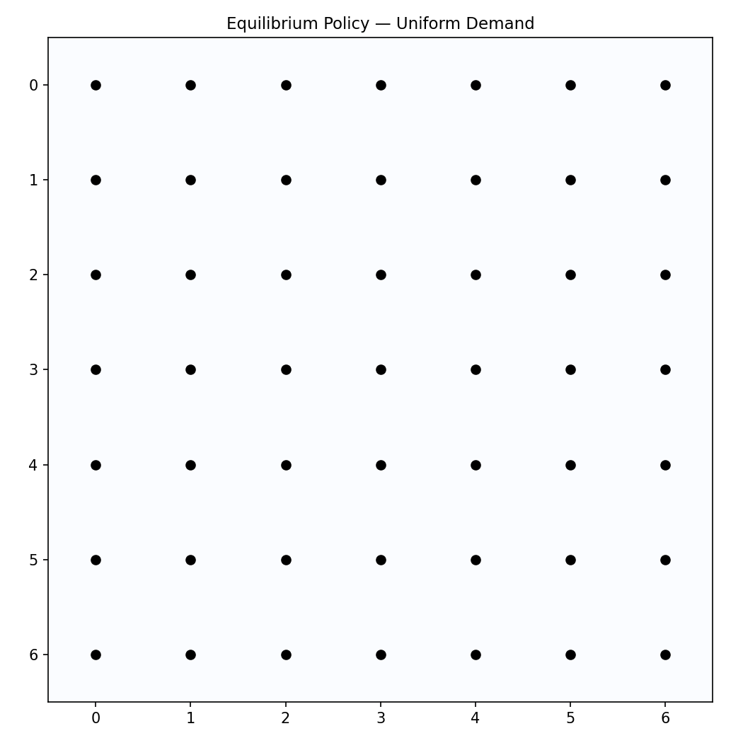
Constant demand everywhere. All zones are equivalent so no spatial selectivity gradient exists. PoA ≈ 1.01 — selfish behavior is nearly optimal.
Demand X[z] — Uniform
Equilibrium idle distribution — perfectly symmetric µ_idle ≈ 0.0045 everywhere
Value function V(z, t=0) — spatially flat, all zones equivalent
Mean acceptance rate — homogeneous, no strategic selectivity
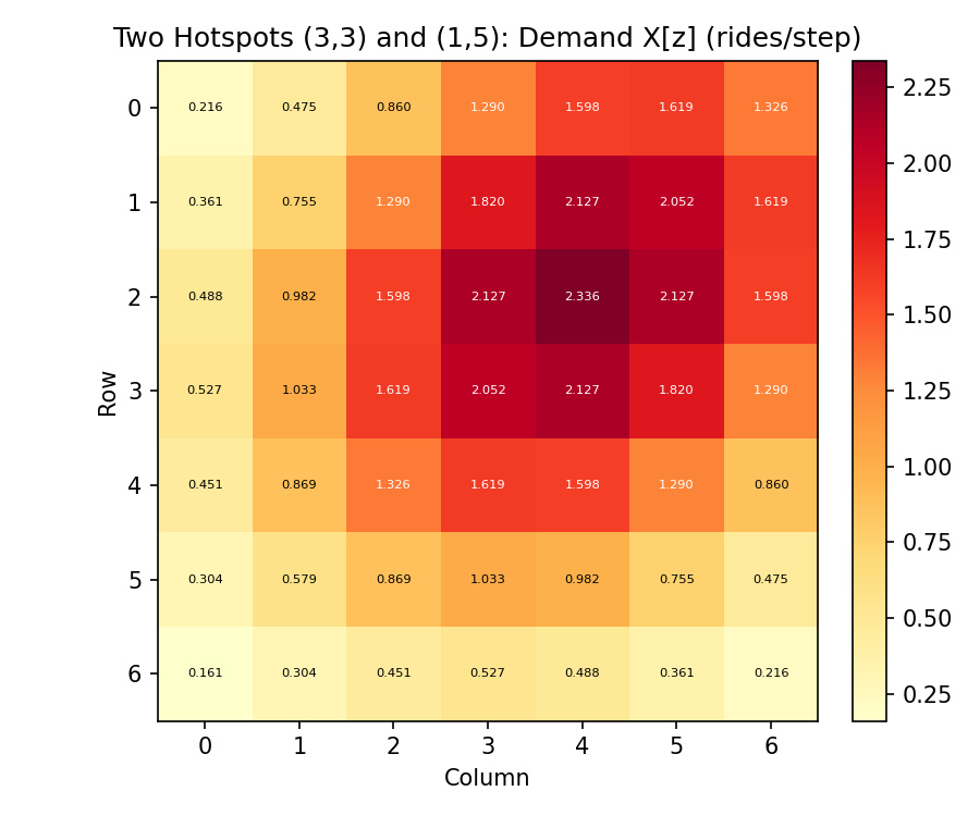
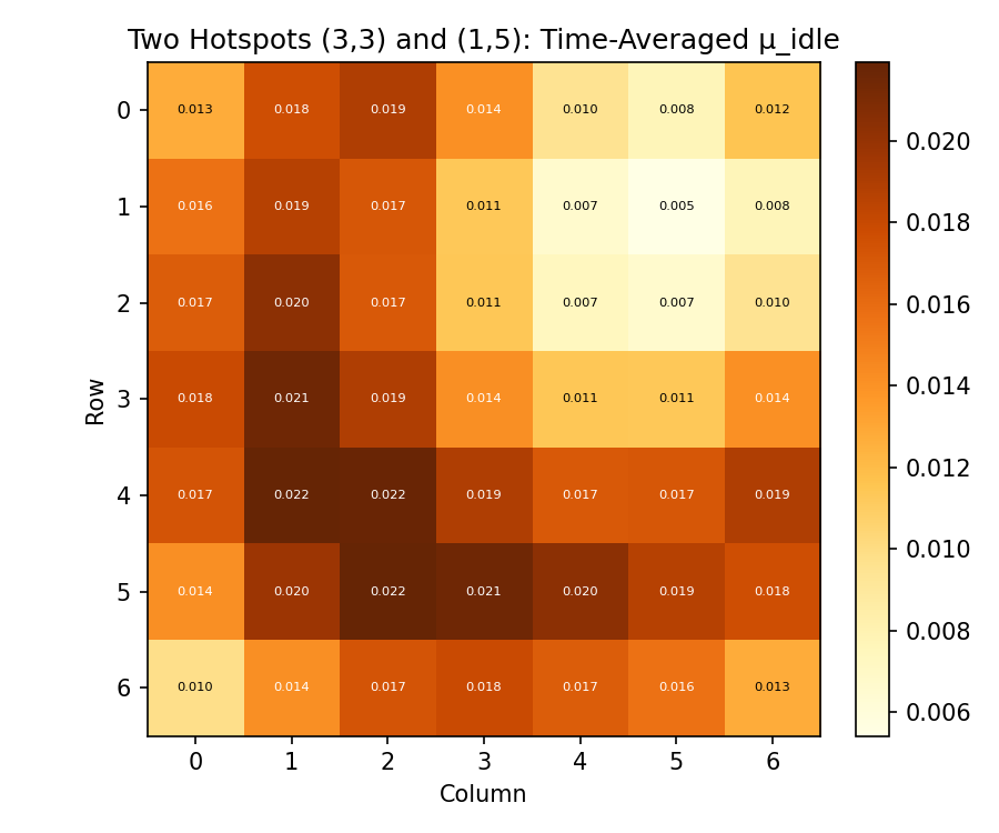
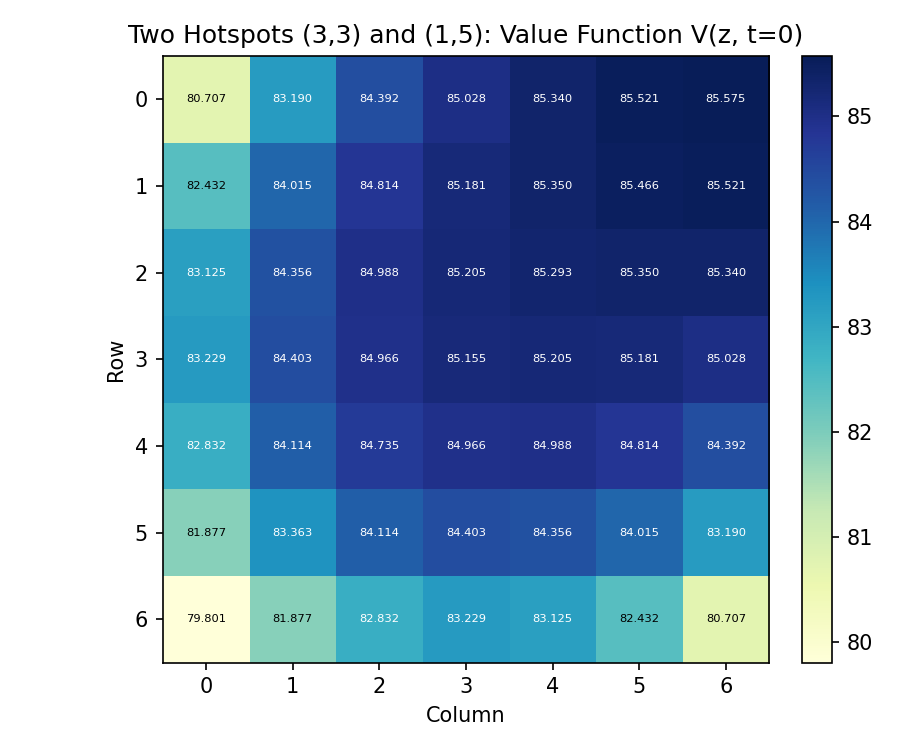
Two Gaussian demand peaks at (3,3) and (1,5). Drivers must choose which center to serve, slightly increasing strategic selectivity. PoA ≈ 1.40.
Demand X[z] — Two Hotspots
Equilibrium idle distribution — two local minima around demand peaks
Value function V(z, t=0) — two high-value regions near demand peaks
Phase 2
Real NYC Data — March 11, 2025
All synthetic assumptions replaced with parameters extracted from real trip records published by the
NYC Taxi & Limousine Commission (TLC) — specifically the High-Volume For-Hire Vehicle
(HVFHV) dataset covering Uber & Lyft rides.
A plain Tuesday, 259 active TLC zones, full minute-level resolution.
259
Active TLC zones
10,979
Estimated drivers
589K
Total rides
166
Iterations to converge
61.6%
Avg busy fraction
76.3%
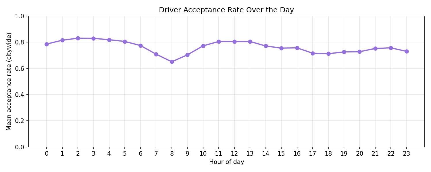
Mean acceptance rate
1.52
Price of Anarchy
JFK
Peak idle zone (zone 132)
✈️
JFK as Peak Idle Zone
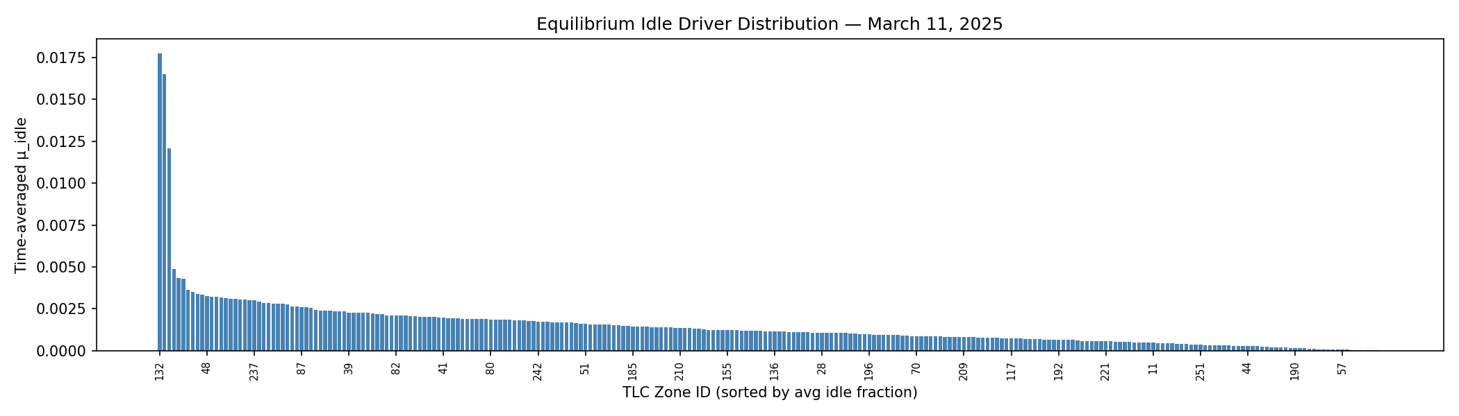
Drivers queue at JFK (zone 132) for high-fare Manhattan runs (~$45–60), accepting longer waits. The TLC even maintains a dedicated driver holding lot here.
🗂️
5-Minute Ride Pool
Phase 2 introduces age cohorts: a rejected ride re-enters the pool for up to 5 minutes before expiring. More realistic than the memoryless Phase 1 model.
🗺️
Empirical O-D Matrix
Destination probabilities P_dest[z,z'] come directly from the data. Most JFK trips go to Midtown — not uniform across 259 zones.
Initialization — Warm Start
µ[z,0] ∝ pickups[z]
proportional to daily trips per zone
→
Always-accept sim
run T=1440 steps
→
Consistent µ[z,t] + R[z,t]
trajectory + ride pool for t=1…1440
Two differences from Phase 1. First, the starting distribution at t=0 is not uniform — drivers are placed proportional to total daily pickups per zone, so high-traffic zones like Midtown start with more drivers than quiet outer-borough zones. Second, Phase 2 also needs to initialize the 5-minute ride pool R[z,t] (the age-cohort backlog of unaccepted rides), not just µ. The always-accept warm start produces both together, giving the outer loop a physically consistent starting point for both the driver distribution and the ride pool.
Convergence
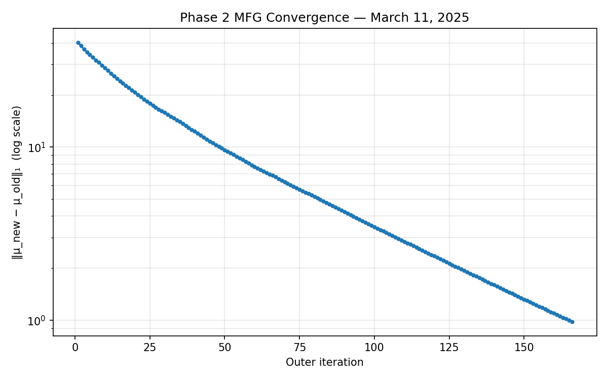
Converged at iteration 166 with final L1 = 0.98. α=0.02 (smaller than Phase 1 to handle spiky real demand). ε=1.0 calibrated to the integer noise floor of real trip counts.
L1 convergence on March 11, 2025 data — converged at iteration 166
Equilibrium Results
Time-averaged idle fraction across 259 zones — JFK (132) dominates, Midtown near zero
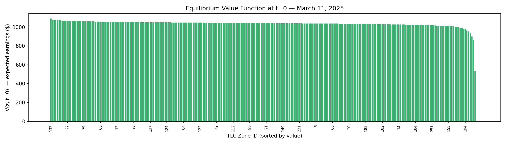
V(z, t=0) — expected full-day earnings by starting zone. Airport zones highest.
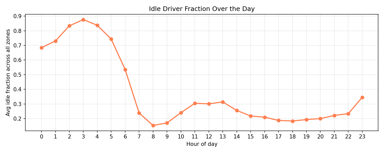
Citywide idle fraction by hour — rush hours (7–9am, 5–8pm) have fewest idle drivers
Citywide mean acceptance rate — drivers most selective during rush hour, near 1.0 at 3am
Phase 1 vs Phase 2
Comparison
Real NYC demand is far spikier than synthetic demand, creating stronger incentives to cluster and widening the gap between selfish and optimal outcomes.
Dimension
Phase 1
Phase 2
Zones
49 synthetic (7×7 grid)
259 real TLC zones
Time horizon
T = 500 steps
T = 1440 minutes (full day)
Demand X[z,t]
Gaussian hotspot (stationary)
Real trip counts (time-varying)
Fare model
γ · Manhattan distance
Median driver_pay from data
Trip duration
Manhattan distance / fixed speed
Median trip_time from data
Destination dist.
Uniform 1/(n−1)
Empirical O-D matrix P_dest
Ride persistence
Discard on reject
5-minute pool (5 age cohorts)
Driver count N
500 (chosen)
10,979 (estimated from data)
α (smoothing)
0.05
0.02
ε (convergence)
0.01
1.0
Iterations
59–139
166
Busy fraction
31.9% (hotspot)
61.6%
Price of Anarchy
≈ 1.37 (hotspot)
1.52
📈
Why is Real-World PoA Higher?
Real NYC demand is spiky — airports and Midtown generate a disproportionate share of trips. This creates stronger clustering incentives, widening the gap between selfish and optimal matching.
🔧
Why Smaller α and Larger ε?
Integer trip counts create a noise floor in the forward simulation. A larger α amplifies this noise causing oscillation. ε=1.0 is calibrated to this floor — it represents genuine convergence, not a loose threshold.
🏙️
34% Welfare Loss
PoA = 1.52 means the selfish equilibrium delivers only 66% of the socially optimal ride matching. A central planner could match 52% more rides with the same number of drivers.
×
What is a Mean-Field Game?
A way to find Nash equilibria when there are too many players to track individually.
The Core Approximation
N players → O(N²) interactions to track
↓ MFG approximation
You only need to track µ, not every other driver
Finding the Equilibrium
µ⁽ᵏ⁾ (mean field)
↓ backward induction → V, π
π* (optimal policy)
↓ forward simulate all drivers
µ̂⁽ᵏ⁺¹⁾ (new distribution)
↓ smooth mix: α·µ̂ + (1−α)·µ
converged? ‖µ_new − µ‖₁ < ε
✓ At convergence: µ* is self-consistent. Playing optimally against µ* reproduces µ*.
Why It Works: Law of Large Numbers
zone 1
zone 2
zone 3
zone 4
zone 5
zone 6
10,979 drivers → their spatial distribution is a smooth, deterministic µ(z,t)
↓
🚕
Each driver is a single atom in a sea. One deviation doesn't move µ — so µ is taken as given.
Nash Equilibrium Condition
π*
best response to µ*
⇄
µ*
distribution induced by π*
If every driver plays π*, the crowd collectively
produces exactly µ* — the distribution π* was
computed against. No one wants to deviate.
In our model: PoA = Wopt / WNash = 1.52 selfish equilibrium = 66% of social optimum